Unit 7: Audio Signal Processing

• Lab 7a
• Lab 7b

• Unit 7 PDF

This unit focuses on processing signals in the audio frequency range using digital signal processing (DSP) concepts with the PIC32MX370 microprocessor. Lab 7a investigates a method of generating multiple frequency signals without using transcendental functions or lookup tables. Lab 7b uses Discrete Fourier Transforms (DFT) to detect the presence of signals. It is not the purpose of this unit to teach the theory of digital filtering, but rather to teach how to implement digital filtering using a conventional microprocessor in lieu of specialized digital signal processors.

• Extend the applications of digital signal processing introduced in Unit 6.
• Use a DSP algorithm to synthesize sine waves.
• Use a DSP algorithm to analyze a periodic signal using Discrete Fourier Transforms.
• How to implement DSP algorithms on the PIC32 processor using C.
• How to use the PIC32 MIPS DSP library to increase the DSP algorithm execution speed.

• Knowledge of C or C++ programming
• Working knowledge of MPLAB® X IDE
• Interfacing with an LCD
• Understanding of Finite Impulse Response Digital Filters
• Understanding of Fourier Transforms

• Basys MX3 trainer board
• Workstation computer running Windows 10 or higher, MAC OS, or Linux
• 2 Standard USB A to micro-B cables

In addition, we suggest the following instruments:

• Analog Discovery 2

The following programs must be installed on your development workstation:

• Microchip MPLAB X® v3.35 or higher
• PLIB Peripheral Library
• XC32 Cross Compiler
• WaveForms 2015 (if using the Analog Discovery 2)
• Iowa Hills Software for IIR and FIR Filters (used for illustrative purposes and is not required)

• How to implement digital filters in C using a PIC32 microprocessor.
• How to create analog output using pulse-width modulation.
• How to sample an analog input at a specified rate.
• How to use the PIC32 processor to make a signal generator.
• How to use the PIC32 processor to make a real-time frequency spectrum analyzer.

As introduced in Unit 6, signal processing is an enabling technology that encompasses the fundamental theory, applications, algorithms, and implementations of processing and transferring information. This information is contained in many different physical, symbolic, or abstract formats broadly designated as signals. In this unit, we will employ both analog and digital signal processing. Analog signal processing will be used to implement frequency filters for both microprocessor inputs and outputs. The analog filters are electronic circuits operating on continuous-time analog signals. Digital filters use computers and microprocessors to perform mathematical operations on sampled, discrete-time signals to reduce or enhance certain aspects of that signal. We looked at how both analog and digital filters are used in open and closed-loop digital control in Labs 6a and 6b. It became apparent that the timing for sampling the inputs and generating the output must occur at fixed intervals.

Analog signal processing is any type of signal processing conducted on continuous analog signals by some analog means. This usually involves electronic circuits consisting of resistors, capacitors, inductors, and high gain differential amplifiers. The term “analog” refers to signals or information that is continuously variable. Mathematically, this implies that the signal can be differentiated an infinite number of times.

Electronic analog computers are able to process analog signals using electronic operational amplifiers to implement the basic mathematical operations such as add, subtract, multiply, and divide transcendental functions such a logarithms and exponentials, as well as integral and differential calculus. Programming analog computers is tantamount to wiring electronic circuits, making them difficult to construct and modify. Although analog computers have been replaced by microprocessors, they are frequently used to implement electronic filters for signal conditioning of digital computer inputs and outputs. Analog filters have the advantage of being able to operate at higher power levels and frequencies.

Digital signal processing (DSP) is the use of digital computers to implement digital processing to perform a wide variety of signal processing operations. The signals processed in this manner are a sequence of numbers that represent samples of a continuous variable in a domain such as time, space, or frequency.

Digital computers, particularly in the form of microprocessors, have replaced the computing effort that was formerly allocated to many analog computers. Digital computers cannot directly process analog input signals without first converting the signal into representations of the signal as discretely varying levels using an analog-to-digital converter (ADC). Digital computers can generate discretely varying output using a digital-to-analog converter (DAC), but to get truly continuous output, the DAC output must be further filtered using an analog filter.

The following discussions provide an outline of the process of designing digital filters. The reader who is interested in an extensive discussion of the field of digital signal processing is directed to Reference 6 that is a PDF book by Steven Smith.

A digital filter is a system that performs mathematical operations on a sampled, discrete-time signal to reduce or enhance certain aspects of that signal. Unit 6, along with Lab 6b, introduces DSP as applies to digital control. In Unit 7, we will apply digital filters to generate and analyze analog signals as modeled in the block diagram in Fig. 6.1.

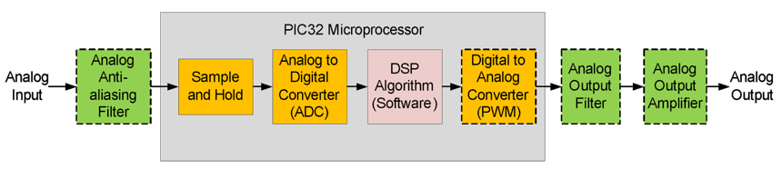Figure 6.1. Block diagram of a digital filter implemented using a microprocessor.

The DSP algorithm repeatedly processes inputs and generates new outputs at a constant rate. This requires sampling and converting the filtered analog input signal at this same rate or a multiple of it. Although the maximum rate that the final DAC analog output can be generated at is the processing rate, outputs can be delayed or generated at lower rates. Unless specifically required, most digital filtering systems sample inputs, process data, and generate output at the same rate. Any variation of the processing rate results in generating incorrect outputs.

Many digital filters are based on design processes utilizing parameters that specify frequency responses in the continuous domain, as expressed with rational polynomials as a function of the Laplace operator “s”. The general form of this polynomial is shown in Eq. 6.1. The study of digital filtering covers the methodologies for determining the specific values for the filter constants $b_j$ and $a_i$ based on the filter criteria.

$$\frac{Y(s)}{X(s)} = H(s) = \frac{\sum_{j=0}^{M-1}b_j \cdots^j}{\sum_{i=0}^{N-1}a_i \cdot s^i} \qquad (\text{Eq. 6.1})$$

Where $Y(s)$ is the system output and $X(s)$ is the system input.

Once the transfer function has been determined that meets the required filter frequency response, the continuous domain transfer function must be approximated by a digital domain transfer function that digital computers can implement as algorithms using programming code. One of the popular approximations is called the bilinear transformation and is expressed by Eq. 6.2.

$$s = \frac{2}{Ts} \frac{1-z^{-1}}{1+z^{-1}} \qquad (\text{Eq. 6.2})$$

Where $Ts$ is the sampling period.

The result of the substitution of Eq. 6.2 into Eq. 6.1 is also a rational polynomial, as shown in Eq. 6.3, that relates the output, $Y(z)$, to the input, $X(z)$. The polynomial coefficients $d_j$ and $c_i$ are not the same values as $b_j$ and $a_i$ used in Eq. 6.1.

$$H(z) = \frac{y(z)}{X(z)} = \frac{FILTERGAIN \cdot \sum_{j-0}^{M-1} d_j \cdot z^{-1}}{1 + \sum_{i=1}^{N-1} c_j \cdot z^{-i}} = \frac{FILTERGAIN \cdot \sum_{j=0}^{M-1} d_j \cdot X(z) \cdot z^{-j}} \qquad (\text{Eq. 6.3})$$

Solving Eq. 6.3 for the output, $Y(z)$, as a function of the input, $X(z)$, results in Eq. 6.4.

$$Y(z) \cdot \bigg[ 1+ \sum_{i=1}^{N-1} c_i \cdot z^{-i} \bigg] = FILTERGAIN \cdot X(z) \cdot \bigg[ \sum_{j=0}^{M-1} d_j \cdot z^{-j} \bigg] \qquad (\text{Eq. 6.4})$$

Using the relationship that the inverse $z$ operator is a delay of one sample, $X(z) \cdot z^{-i}$ becomes $x(n-i)$. Hence, Eq. 6.5 is the inverse $z$ transform of Eq. 6.3.

$$y(n) + \sum_{i=1}^{N-1

—-